Initializing the Satellite Galaxy

The satellite galaxy comprises two key components: the galaxy potential as well as the particle distribution which is actually what GalaRP uses to trace orbits.

The Satellite Galaxy Potential

The satellite galaxy potential can be any combination of Gala potentials. For example:

import gala.potential as gp

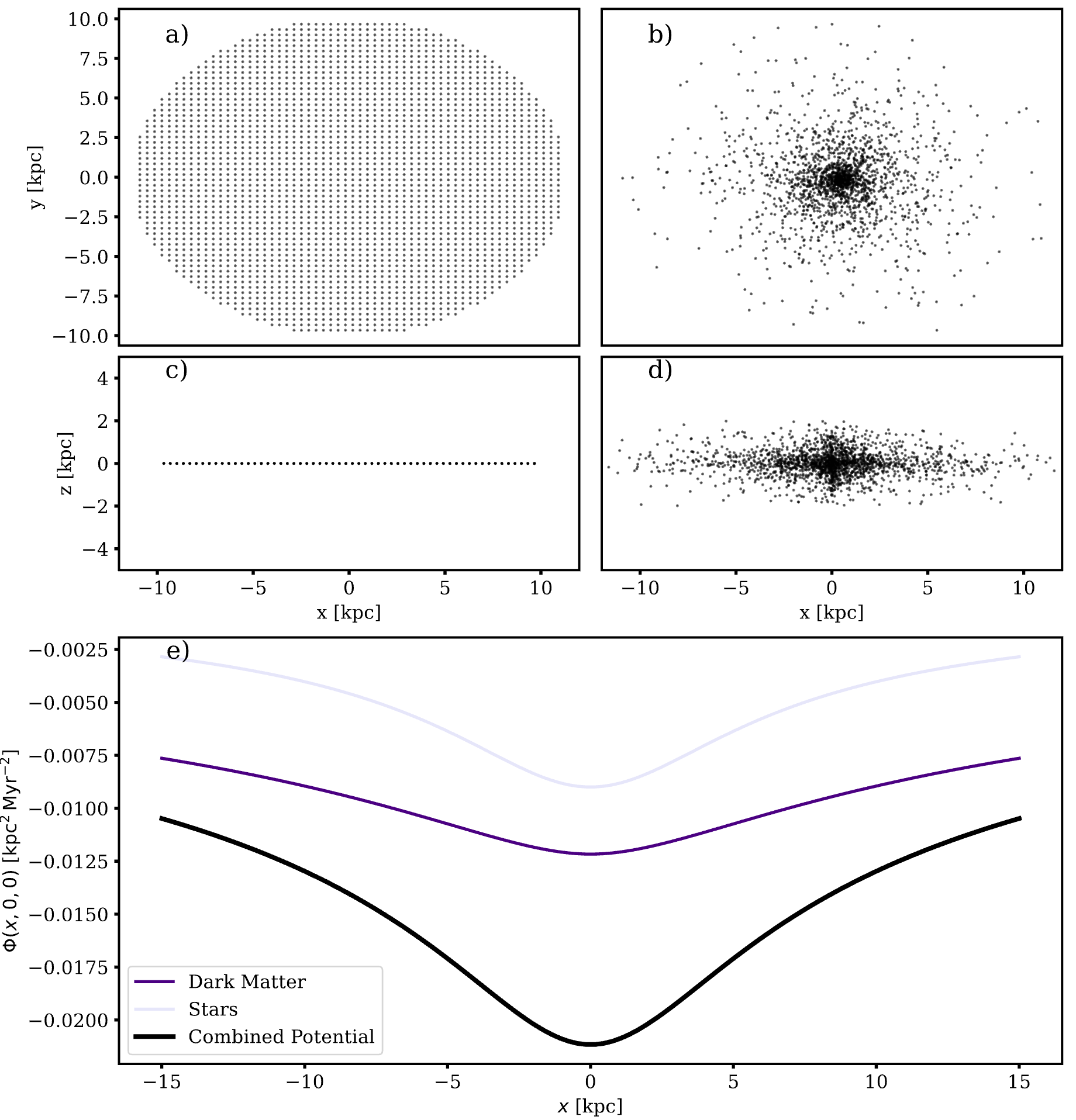
dm = gp.BurkertPotential(rho=5.93e-25 * u.g / u.cm**3, r0=11.87 * u.kpc, units=galactic)

stars = gp.MiyamotoNagaiPotential(m=10**9.7 * u.Msun, a=2.5 * u.kpc, b=0.5 * u.kpc, units=galactic)
gas = gp.MiyamotoNagaiPotential(m=10**9.7 * u.Msun, a=3.75 * u.kpc, b=0.75 * u.kpc, units=galactic)

pot = gp.CompositePotential(dm=dm, stars=stars, gas=gas)

In this case we return an explicit composite potential, where you can access the components easily using pot["dm"], for example.

GalaRP also has built-in potentials under the builtins.satellites module.

Note that a GalaRP-defined mass profile should be generated using the following:

mass_profile = grp.gen_mass_profile(pot)

Particle Initialization

To run a GalaRP sim, the user needs to define some set of particles through which the RP orbits are calculated. The main particle classes included are a uniform grid of equally spaced particles, as well as a particle distribution matching the density distribtion of a double-exponential model:

\[n(R,z) = n(0, 0)\exp\left(-\frac{R}{h_R}\right)\exp\left(-\frac{|z|}{h_z}\right)\]

For a uniform grid with a maximum radius of 10 kpc:

particles = grp.UniformGrid(n_particles=150, Rmax=10)
particles.generate(mass_profile=mass_profile)

This will create a uniform grid with 50 particles from -Rmax to Rmax. It will also automatically initialize the particles with a velocity dispersion of 10 km/s along each axis.